Using Google Analytics & Google Trends API to Track Performance with R

Danny Smith ● December 15, 2021 | Analytics

Written by Danny Smith
December 15, 2021 | Analytics

Why is Google Trends Data Powerful?

We all know that Google captures a frightening amount of data about us. With billions of searches each day, Google can understand a lot more about our society and the sentiment of populations than governments. For example, search trends data can recognise disease outbreaks far before they are announced by the media by seeing increases in search queries related to specific symptoms. Unsurprisingly, studies have been carried out to forecast rising COVID-19 cases by region.

These days, Google is essentially the world’s sentiment barometer and the best thing about Google’s search trend data? It’s free.

Why use the Google Trends API?

Google Trends is a key feature of many digital marketer’s toolkit. The popularity of search queries over time can be analysed to show market awareness. Overlaying this data with that of other sources can provide insights that would otherwise be missed.

This blog provides such an example by showing how you can overlay Google Trends data with your website’s organic traffic – this can be used to understand SEO performance. If your organic traffic is beginning to slip, is this due to a drop in market interest or because you aren’t ranking so highly for your top search queries?

There are R packages available for both Google Trends and Google Analytics which are pretty easy to use for those with a basic understanding of programming. For Google Trends we will use the gtrendsR package and then for Google Analytics we will use the googleAnalyticsR package, which we covered in our previous article – Using the Google Analytics API with R. The example code provided should be straightforward to copy/paste and adapt to suit your needs.

We will use the example of a company that sells soft drinks and is wanting to understand the popularity over time of products they sell.

Google Trends API – How to Pull Search Trends Data

This data is the easiest to obtain, mainly because there are no API keys required. To start, simply install the package with install.packages(“gtrendsR”) and load up the library with library(gtrendsR). Selecting the desired keywords can be difficult – we recommend looking at the top non-brand terms in Search Console ordered by impressions.

# Load Libraries and Set Up Query Conditions #

library(gtrendsR)
keywords = c(“Soft drinks”, “Fizzy drinks”, “Pepsi”, “Lemonade”, “Fanta”)
country = c(‘GB’)
time = (“2020-01-01 2021-10-31”)
channel = ‘web’
# Run Query #
data1 = gtrends(keywords, gprop = channel, geo = country, time = time)
data_trend = data$interest_over_time

As shown in the above code, additional variables can be included in your request: gprop, geo and time:

Gprop represents Google’s properties, namely news, images and YouTube – however if left blank this will default to web.
Geo represents the country based on their two digit ISO code – however if left blank this will default to worldwide.
Time represents the start and end date of the request.

The gtrendsR package has a limit of 5 keywords at a time, so if you want to run multiple queries then you can use a loop as shown below. We advise doing this if you are assessing the overall popularity of a collective of search terms, as this loop runs each keyword separately before aggregating each of their weekly changes. Therefore, the change in popularity of one has no direct impact on that of another.

list1 = list()
for (i in 1:length(keywords)){
  trends = gtrends(keywords[i], gprop =channel,geo=country, time = time )
  time_trend=trends$interest_over_time
  time_trend$keyword <- keywords[i]
  list1 [[i]] <- time_trend
}
data1 <- do.call("rbind", list1)

One thing to note is that Google Trends provides weekly data, but the weeks start on a Sunday. Therefore, we will need to aggregate our Google Analytics data at week-level starting on a Sunday – there is a useful package to help us do this that we will cover later.

Google Analytics API – How to Pull Organic Traffic

We recommend reading our previous article to understand the googleAnalyticsR package in more detail. This article shows you how you can filter your organic traffic to specific landing pages. This might be useful if your company is in multiple markets. i.e. If you sell fizzy drinks and chocolate bars then you would not want to include the organic traffic to the chocolate bars pages when assessing the market interest of fizzy drinks.

Otherwise, the code below allows you to access all your site’s organic traffic using this package with R.

We advise running each line of a code at a time so you can easily spot any errors.

For a more ‘professional’ way of authentication, which helps with script automation, have a look at this more detailed explanation.

The below code pulls organic traffic by day. The floor_date function is then used to aggregate the traffic by week starting on Sunday, in order to match the Search Console data (which is limited to weekly data Sun-Sat).

# Load Libraries and Setup Query - make sure to set your View ID #
library(googleAnalyticsR)
library(dplyr)
library(lubridate)
ga_auth()
set_view_ID <- #ENTER_VIEW_ID#
organicTraffic <- dim_filter("channelGrouping", "EXACT", "Organic Search")
organicFilter <- filter_clause_ga4(list(organicTraffic),”AND” ) 
# Run Query, Aggregate Daily Traffic to Weekly Traffic and Rename Columns #
data2 <- google_analytics (set_view_ID,
                          date_range = c(“2021-01-01”, ”2021-10-31”),
                          metrics = "sessions",
                          dimensions = "date",
                          dim_filters = organicFilter, 
                          anti_sample = TRUE)

data2$week <- floor_date(as.Date(data2$date, "%Y-%m-%d"), unit="week")


data2 <- data2 %>% group_by(week) %>% summarise(sum(sessions))
names(data2)[1] <- "week"
names(data2)[2] <- "sessions"

# Merge Search Trends and Organic Traffic # 

merged_data <- merge(data1, data2)

Merging the Datasets and Gaining Insights

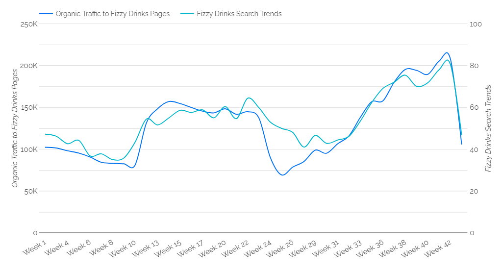
In our final line of code above, we have merged the datasets together into 3 columns: week start date, organic sessions and relative search trend. Now these two datasets can easily be overlayed in a graph to analyse (see graph below for example).

The aggregation of the Search Trends data means that we can see the relative popularity across all search queries over time, providing an insight into the changes in market interest.

We recommend overlaying the Search Trends data and organic traffic on a graph over time using a right and left axis in order to assess the trend. What you will likely see is a positive correlation between them, with traffic increasing as search popularity increases. There may be points where the lines deviate from another, indicating a change in keyword rankings. Does it look like you are moving up or down Google’s search results page?

The graph below shows example data with the organic traffic on the left axis and the search trends on the right axis. In the graph below there is clear divergence between the two metrics in week 24. Despite the organic traffic dropping significantly, the search trends stays relatively consistent, indicating a drop in keyword rankings to the pages that drive high-volume of traffic – these rankings then pick up towards week 33.

This is just one use case of the Search Console API. It has numerous other roles to play in the marketing space, such as generating live search term trends reports which can be used for reactive digital PR stories, or observing the brand popularity of competitors overtime.

Keen to know more? Contact us to speak to someone in our advanced web analytics team!